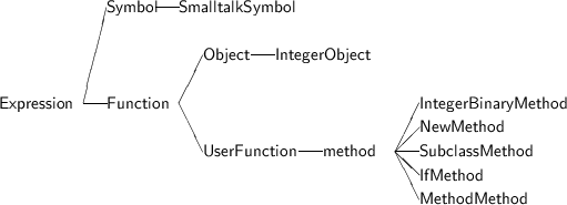
Figure 1.1: The Expression class Hierarchy in Chapter 1
________________________________________________________________________________________________________________________________________________________
The Kamin Interpreters in C++
_____________________________________________________________________________________________________________
This paper describes C++ implementations of the interpreters in the book
\Programming Languages: An Interpreter-Based Approach"
by Samuel Kamin (Addison-Wesley, 1989).
Timothy Budd
September 11, 1991
Updated by Henry G. Weller
January 25, 2014
Abstract
This paper describes a series of interpreters for the languages used in the book \Programming Languages: An Interpreter-Based Approach" by Samuel Kamin (Addison-Wesley, 1989). Unlike the interpreters provided by Kamin, which are written in Pascal, these interpreters are written in C++. It is my belief that the use of inheritance in C++ better illustrates the unique features of each of the several languages. In the Pascal versions of the interpreters the di�erences between the various interpreters, although small, are scattered throughout the code. In the C++ versions di�erences are produced using only the mechanism of subclassing. This means that the vast majority of code remains the same, and di�erences can be much more precisely isolated.
The chapters in this report correspond to the chapters in the original text. Where motivational or background material is provided in that source it is generally omitted here. A major exception is in those places (chie�y chapters 3, 7 and 8) where I have selected a syntax slightly di�erent from that provided by Kamin.
The use of an Object-Oriented language for the interpreters may seem a bit incongruous, since Object-Oriented programming is not discussed until Chapter 7. Nevertheless, I think the bene�ts of programming the interpreters in C++ outweighs this problem.
The structure of our basic interpreter1 di�ers somewhat from that described by Kamin. Our interpreter is structured around a small main program which manipulates three distinct types of data structures. The main program is shown in Figure 1.1, and will be discussed in more detail in the next section. Each of the three main data structures is represented by a C++ class, such is subclassed in various ways by the di�erent interpreters. The three varieties of data structures are the following:
In subsequent sections we will explore in more detail each of these data structures.
Figure 1.1 shows the main program, 2 which de�nes the top level control for the interpreters. The same main program is used for each of the interpreters. Indeed, the vast majority of code remains constant throughout the interpreters.
The structure of the main program is very simple. To begin, a certain amount of initialization is necessary. There are four global variables found in all the interpreters. The variable emptyList contains a list with no elements. (We will return to a discussion of lists in Section 1.4.4). The three environments globalEnvironment, valueOps and commands represent the top-level context for the interpreters. The globalEnvironment contains those symbols that are accessible at the top level. The valueOps are those operations that can be performed at any level, but which are not symbols themselves that can be manipulated by the user. Finally commands are those functions that can be invoked only at the top level of execution. That is, commands cannot be executed within function de�nitions.
Following the common initialization the function initialize is called to provide interpreter-speci�c initialization. This chie�y consists of adding values to the three environments. This function is changed in each of the various interpreters.
The heart of the system is a single loop, which executes until the user types the directive quit.3 The reader (which must be de�ned as part of the interpreter-speci�c initialization) requests a value from the user. After testing for the the quit directive, the entered expression is evaluated. We will defer an explaination of the evalAndPrint method until Section 1.4, merely noting here that it evaluates the expression the user has entered and prints the result. The read-eval-print cycle then continues.
Readers are implemented by instances of class Reader, shown in Figure 1.2. The only public function performed by this class is provided by the method promptAndRead, which prints the interpreter prompt, waits for input from the user, and then parses the input into a legal, but unevaluated, expression (usually a symbol, integer or list-expression). These actions are implemented by a variety of utility routines, which are declared as protected so that they may be made available to later subclasses.
The code that implements this data structure is relatively straight-forward, and most of it will not be presented here. The main method is the single public-accessible routine promptAndRead, which is shown in Figure 1.3. This method loops until the user enters an expression. The method �llInputBu�er places the instance pointer p at the �rst non-space character (also stripping out comments). Thus lines containing only spaces, newlines, or comments are handled quickly here, and cause no further action. Also, as have noted previously, an end-of-input indication is caught by the method �llInputBu�er, which then places the quit command in the input bu�er. The method readExpression (Figure 1.4) is the parser used to break the input into an unevaluated expression. This method is declared virtual, and thus can be rede�ned in subclasses. The base method recognizes only integers, symbols, and lists. The routine to read a list recursively calls the method to read an expression.
As we have noted already, the Environment data structure is used to maintain symbol-value pairings. In addition to the global environments de�ned during initialization, environments are created for argument lists passed to functions, and in various other contexts by some of the later interpreters. Environments can be linked together, so that if a symbol is not found in one environment another can be automatically searched. This facilitates lexical scoping, for example.
For reasons having to do with memory management, the Environment data structure, shown in Figure 1.5, is declared as a subclass of the class Expression. Unlike other expressions, however, environments are never directly manipulated by the user. Also for memory management reasons, there is a class Env declared which can maintain a pointer to an environment. The two methods de�ned in class Env set and return this value. Anytime a pointer is to be maintained for any period of time, such as the link �eld in an environment, it is held in a variable declared as Env rather than as a pointer directly. Finally the overridden virtual methods isEnvironment and free in class Environment are also related to memory management, and we will defer a discussion of these until the next section.
The three methods used to manipulate environments are lookup, add and set. The �rst attempts to �nd the value of the symbol given as argument, returning a null pointer if no value exists. The method add adds a new symbol-value pair to the front of the current environment. The method set is used to rede�ne an existing value. If the symbol is not found in the current environment and there is a valid link to another environment the linked environment is searched. If the link �eld is null (that is, there is no next environment), the symbol and valued are added to the current environment.
Environments are implemented using the List data structure, a form of Expression we will describe in more detail in Section 1.4.4. Two parallel lists contain the symbol keys and their associated values. For the moment it is only necessary to characterize lists by four operations. A list is composed of list nodes (elements of class ListNode). Each node contains an expression (the head) and, recursively, another list. The special value emptyList, which we have already encountered, terminates every list. The operation head returns the �rst element of a list node. When provided with an argument, the operation head can be used to modify this �rst element. The operation tail returns the remainder of the list. Finally the operation isNil returns true if and only if the list is the empty list.
Figure 1.6 shows the method lookup, which is de�ned in terms of these four operations. The while loop cycles over the list of keys until the end (empty list) is reached. Each key is tested against the argument key, using the equality test provided by the class Symbol. Once a match is found the associated value is returned.
If the entire list of names is searched with no match found, if there is a link to another environment the lookup message is passed to that environment. If there is no link, a null value is returned.
The routine to add a new value to an environment (Figure 1.7) merely attaches a new name and value to the beginning of the respective lists. Note by attaching to be beginning of a list this will hide any existing binding of the name, although such a situation will not often occur. The method set searches for an existing binding, replacing it if found, and only adding the new element to the �nal environment if no binding can be located.
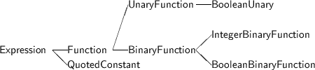
The class Expression is a root for a class hierarchy that contains the majority of classes de�ned in these interpreters. Figure 1.1 shows a portion of this class hierarchy. We have already seen that environments are a form of expression, as are integers, symbols, lists and functions.
The major purposes of the abstract class Expression (Figure 1.8) are to perform memory management functions, to permit conversions from one type to another in a safe manner, and to de�ne protocol for evaluation and printing of expression values. The latter is easist to dismiss. The virtual methods eval and print provide for evaluation and printing of values. The eval method takes as argument a target expression to which the evaluated expression will be assigned, as well as two environments. The �rst environment contains the list of legal value-ops for the expression, while the second is the more general environment in which the expression is to be evaluated. The default method for eval merely assigns the current expression to the target. This su�ces for objects, such as integers, which yield themselves no matter how many times they are evaluated. The default method print, on the other hand, prints an error message. Thus this method should always be overridden in subclasses.
For long running programs it is imperative that memory associated with unused expressions be recovered by the underlying operating system. This is accomplished in these interpreters through the mechanism of reference counts. Every expression contains a reference count �eld, which is initially set to zero by the constructor in class Expression. The integer value maintained in this �eld represents the number of pointers that reference the object. When this count becomes zero, no pointers refer to the object and the memory associated with it can be recovered.
The maintenance of reference counts if peformed by the class Expr (Figure 1.9). As with the class Env we have already encountered, the class Expr is a holder class, which maintains an expression pointer. A value can be inserted into an Expr either through construction or the assignment operator. A value can be retrieved either though the protected method val or, as a notational convenience, through the parenthesis operator. The method evalAndPrint, as have noted already, merely passes the eval message on to the underlying expression and prints the resulting value.
Figure 1.10 gives the implementation of the constructor and assignment operator for class Expr. The constructor takes an optional pointer to an expression, which may be a null expression (the default). If the expression is non-null, the reference count for the expression is incremented. Similarly, the assignment operator �rst increments the reference count of the new expression. Then it decrements the reference count of the existing expression (if non-null), and if the reference count reaches zero, the memory is released, using the system function delete. Immediately prior to destruction, the virtual method free is invoked. Classes can override this method to provide any necessary class-speci�c maintenance. For example, the class Environment (Figure 1.5) assigns null values to the structures theNames, theValues and theLink, thereby possibly triggering the release of their storage as well.
A common di�culty in a statically typed language such as C++ is the container problem. Elements placed into a general purpose data structure, such as a list, must have a known type. Generally this is accomplished by declaring such elements as a general type, such as Expression. But in reality such elements are usually instances of a more speci�c subclass, such as an integer or a symbol. When we remove these values from the list, we would like to be able to recover the original type.
There are actually two steps in the solution of this problem. The �rst step is testing the type of an object, to see if it is of a certain form. The second step is to legally assign the object to a variable declared as the more speci�c class. In these interpreters the mechanism of virtual methods is used to combine these two functions. In the abstract class Expression a number of virtual functions are de�ned, such as isInteger and isEnvironment. These are declared as returning a pointer type. The default behavior, as provided by class Expression, is to return a null pointer. In an appropriate class, however, this method is overridden so as to return the current element. That is, the class associated with integers overrides isInteger, the class associated with symbols overrides isSymbol, and so on. Figure 1.2 shows the two de�nitions of isEnvironment, the �rst from class Expression and the second from class Environment. By testing whether the result of this method is non-null or not, one can not only test the type of an object but one can assign the value to a speci�c class pointer without compromising type safety. An example bit of code is provided in Figure 1.2 that illustrates the use of these functions.
The method touch presents a slightly di�erent situation. It is de�ned in the abstract class to merely return the object to which the message is sent. That is, it is a null-operation. In Chapter 5, when we introduce delayed evaluation, we will de�ne a type of expression which is not evaluated until it is needed. This expression will override the touch method to force evaluation at that point.
Internally within the interpreters integers are represented by the class IntegerExpression (Figure 1.11). The actual integer value is maintained as a private value set as part of the construction process. This value can be accessed via the method val. The only overridden methods are the print method, which prints the integer value, and the isInteger method, which yields the current object.
Symbols are used to represent uninterpreted character strings, for example identi�er names. Instances of class Symbol (Figure 1.12) maintain the text of their value in a private instance variable. This character pointer can be recovered via the method chars. Storage for this text is allocated as part of the construction process, and deleted by the virtual method free. The equality testing operators return true if the current symbol matches the text of the argument.
Figure 1.12 also shows the implementation of the method eval in the class Symbol. When a symbol is evaluated it is used as a key to index the current environment. If found the (possibly touched) associated value is assigned to the target. If it is not found an error message is generated. The routine error always yields a null expression.
We have already encountered the behavior of the List data structure (Figure 1.13) in the discussion of environments. As with expressions and environments, lists are represented by a pair of classes. The �rst, class ListNode, maintains the actual list data. The second, class List, is merely a pointer to a list node, and exists only to provide memory management operations.
Only one feature of the latter class deserves comment; rather than overloading the parenthesis operator the class List de�nes a conversion operator which permits instances of class List to be converted without comment to ListNodes. Thus in most cases a List can be used where a ListNode is expected, and the conversion will be implicitly de�ned. We have seen this already, without having noted the fact, in several places where the variable emptyList (an instance of class List) was used in situations where an instance of class ListNode was required.
The actual list data is maintained in the instance variables h and t, which we have already noted can be retrieved (and, in the case of the h, set) by the methods head and tail. The method length returns the length of a list, and the method at permits a list to be indexed as an array, starting with zero for the head position.
The majority of methods, such as length, at, print, are simple recursive routines, and will not be discussed. Only one method is su�ciently complex to deserve comment, and this is the procedure used to evaluate a list. A list is interpreted as a function call, and thus the evaluation of a list involves �nding the indicated function and invoking it, passing as arguments the remainder of the list. These actions are performed by the method eval shown in Figure 1.14. An empty list always evaluates to itself. Otherwise the �rst argument to the list is examined. If it is a symbol, a test is performed to see if it is one of the value-ops. If it is not found on the value-op list the �rst element is evaluated, whether or not it is a symbol. Generally this will yield a function value. If so, the method apply, which we will discuss in the next section, is used to invoke the function. If the �rst argument did not evaluate to a function an error is indicated.
If expressions are the heart of the interpreter, then functions are the muscles that keep the heart working. All behavior, statements, valueops, as well as user-de�ned functions, are implemented as subclasses of class Function (Figure 1.15). As we noted in the last section, when a function (written as a list expression) is evaluated the method apply (Figure 1.16) in invoked. This method takes as argument the target for the evaluation and a list of unevaluated arguments. The default behavior in class Function is to evaluate the arguments, using the simple recursive routine evalArgs, then invoke the method applyWithArgs.
Both the methods apply and applyWithArgs are declared as virtual, and can thus be overridden in subclasses. Those function that do not evaluate their arguments, such as the functions implementing the control structures of Chapter 1, override the apply method. Function that do evaluate their arguments, such as the majority of value-Ops, override the applyWithArgs method.
Two subclasses of Function deserve mention. The class UnaryFunction overrides apply to test that only one argument has been provided. Similarly the class BinaryFunction tests for exactly two arguments. The remaining major subclass of Function is the class UserFunction. We will defer a discussion of this until we examine the implementation of the de�ne statement.
We are now in a position to �nally describe the characteristics that are unique to the basic evaluator of chapter one. This interpreter recognizes one command (the de�ne statement), several built-in statements (if, while, set, and begin), and a number of value-ops. All are implemented internally as functions. What syntactic category a symbol is associated with is determined by what environment it is placed on, and not by the structure of the function.
The de�ne statement is implemented as the single instance of the class De�neStatement (Figure 1.17), entered with the key \de�ne" in the commands environment. The class overrides the virtual method apply (Figure 1.18), since it must access its arguments before they are evaluated. It tests that the arguments are exactly three in number, and that the �rst is a symbol and the second a list. If no errors are detected, an instance of the class UserFunction is created and and set in the current (always global) environment.
The class UserFunction created by the de�ne statement is similarly a subclass of class Function (Figure ??). User functions maintain in instance variables the list of argument names, the body of the function, and the lexical context in which they are to execute. These values are set by the constructor when the function is de�ned, and freed by the virtual method free when no longer needed.
User functions always work with evaluated arguments, and thus they override the method applyWithArgs. The implementation of this method is shown in Figure ??. This method checks that the number of arguments supplied matches the number in the function de�nition, then creates a new environment to match the arguments and their values. The expression which represents the body of the function is then evaluated. By passing the new context as argument to the evaluation, symbolic references to the arguments will be matched with the appropriate values.
The built-in statements if, while, set and begin are each de�ned by functions entered in the valueOps environment. With the exception of begin, these must capture their arguments before they are evaluated and thus, like de�ne, they override the method apply.
The If statement (Figure ??, Figure ??) �rst insures it has three arguments. It then evaluates the �rst argument. Using the auxiliary function isTrue (Figure 1.23) (which will vary over the di�erent interpreters as our de�nition of \true" changes) the truth or falsity of the �rst expression is determined. Depending upon the outcome, either the second or third argument is evaluated to determine the result. In the Chapter 1 interpreter the value 0 is false, and all other values (integer or not) are considered to be true.
The function that implements the while statement is shown in Figure 1.24. Although the while statement requires two arguments, it nevertheless cannot usefully be made a subclass of class BinaryFunction, since it must access its arguments before they are evaluated. The implementation of the while statements loops until the �rst argument evaluates to a true condition, using the same test for true method used by the if statement. The results returned by evaluating the body of the while statement are ignored, as the body is executed just for side e�ects.
The implementation of the set statement is shown in Figure 1.25. The function insures the �rst argument is a symbol, evaluates the second argument, then sets the binding of the symbol to value in the current environment.
The begin statement evaluate each of its arguments and assigns to the target variable the value of the last expression (Figure 1.26).
The Value-ops are functions placed in the valueop global environment. They can be divided into two categories; there are those that take two integer arguments and produce an integer result (+, �, �, =, =, < and >) and those that take a single argument (print).
The implementation of the integer binary functions is simpli�ed by the introduction of an intermediate class IntegerBinaryFunction, a subclass of BinaryFunction (Figure 1.28). The private state for each instance of this class holds a pointer to a function that takes two integer values and generates an integer result. The applyWithArgs method in this class decodes the two integer arguments, then invokes the stored function to produce the new integer value. To implement each of the seven binary integer functions (the relational functions generate 0 and 1 values for true and false, remember) it is only necessary de�ne an appropriate function and pass it as argument to the constructor during initialization of the interpreter. This can be seen in Figure 1.31.
The print function is implemented by a subclass of UnaryFunction that merely invokes the method print on the argument. All expressions will respond to this method.
Figure 1.31 shows the initialization routine for the interpreters of chapter one. In chapter one there are no global variables de�ned at the start of execution. There is one command, the statement de�ne, and a number of value-ops.
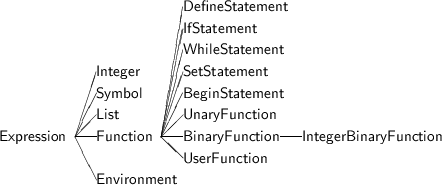
The interpreter for Lisp di�ers only slightly from that of Chapter one. The reader/parser is modi�ed so as to recognize quoted constants, two new global variables (T and nil) are added, and a number of new value-ops are de�ned. In all other respects it is the same. Figure 2.1 shows the class hierarchy for the expression classes added in chapter 2.
The Lisp reader is created by subclassing from the base class Reader (Figure 2.1). The only change is to modify the method readExpression to check for leading quote marks. If no mark is found, execution is as in the default case. If a quote mark is found, the character pointer is advanced and the following expression is turned into a quoted constant. Note that no checking is performed on this expression. This permits symbols, even separators, to be treated as data. That is, '; is a quoted symbol, even though the semicolon itself is not a legal symbol.
To create quoted constants it is necessary to introduce a new type of expression. When an instance of class QuotedConst is evaluated, it simply returns its (unevaluated) data value.
In addition to adding a number of new value-ops, the Lisp interpreter modi�es the meaning of a few of the Chapter 1 functions. For example the relational operators must now return the values T or nil, and not 1 and 0 values. Similarly the meaning of true and false used by the if and while statements is changed. Finally the equality testing function (=) must now recognize both symbols and integers.
Figure 2.3 shows the revised de�nition of the equality testing function, which now must be prepared to handle symbols and well as integers.
Implementation of the boolean binary functions is simpli�ed by the introduction of a class BooleanBinaryFunction (Figure 2.4). This class decodes the two integer arguments and invokes a further method to determine the boolean result. Based on this result either the value of the global symbol representing true or the symbol representing false is returned.
Finally Figure 2.6 shows the revised function used by if and while statements to determine the truth or falsity of their condition. Unlike in Chapter 1, where 0 and 1 were used to represent true and false, here nil is used as the only false value.
car and cdr are implemented as simple unary functions (Figure 2.7), and cons is a simple binary function that creates a new ListNode out of its two arguments.
The implementation of the predicates number?, symbol?, list? and null? is simpli�ed by the creation of a class BooleanUnary (Figure 2.8), subclassing UnaryFunction. As with the integer functions implemented in chapter 1, instances of BooleanUnary maintain as part of their state a function that takes an expression and returns an integer (that is, boolean) value. Thus for each predicate it is only necessary to write a function which takes the single argument and returns a true/false indication.
Figure 2.10 shows the initialization method for the Lisp interpreter.
My version of the APL interpreter di�ers somewhat from that provided by Kamin:
Despite the APL interpreter being larger than any other interpreter, I think that the addition of a few more functions could give the student an even better feel for the language, as well as providing a smooth transition to functional programming. Speci�cally, I think reduction should be de�ned as a functional, and inner and outer products added as operations. I have not done this as yet, however.
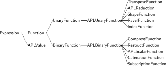
Figure 3.1 shows the class hierarchy for the classes introduced in this chapter.
The APL interpreter manipulates APL values, which are de�ned by the data type APLValue (Figure 3.1). An APL value represents a integer rectilinear array. Internally, such a value is represented by a list that maintains the shape (extent along each dimension) and a vector of integer values. The length of the shape list provides the rank (dimensionality) of the data value. The product of the values in the shape indicates the number of elements in the array, except in the case of scalar values, which have an empty shape array.
APL values are stored in what is called ravel-order. This is what in some other languages is called row-major order.
The methods de�ned for APL values can be used to determine the number of elements contained in the structure (size), obtain the shape of the value (shape), obtain the shape at any given dimension (shapeAt), obtain the value at any given ravel-order position (at), and �nally change the value at any position (atPut).
The APL reader is modi�ed so that individual scalar values and vectors of integers are recognized as APL values. The class de�nition for APLreader is shown in Figure 3.2, and the code for the two auxiliary functions in the next �gure.
The implementation of the APL functions is simpli�ed by the addition of two auxiliary classes, APLUnary and APLBinary. In addition to checking that the right number of arguments are provided to a function application, these check to insure that the arguments are APL values 1 and invoke yet another virtual function applyOp, to perform the actual calculation.
By far the largest class of APL functions are the so-called scalar functions. These are the conventional arithmetic and logical functions, such as addition and multiplication, extended in the natural way to arrays. The only complication in the implementation of these values concerns what is called scalar extension. That is, a scalar value can be used as either the left or right argument to a scalar function, and it is treated as if it were an entire array of the correct dimensionality to match the other argument. Since scalar extension can occur with either the left or right argument, the code for scalar functions divides naturally into three cases.
Scalar functions are implemented using a single class by making use, as we have done before, of an instance variable that contains a pointer to a integer function that generates an integer result. The class APLscalarFunction and the method applyOp are shown in Figure 3.4. Note that the same functions used in the previous interpreters can be used in the construction of the APL scalar functions.
For each scalar function there is an associated reduction function.2 Reduction in these interpreters always occurs along the last dimension. Thus to compute the size of a new value is su�ces to remove the last dimension value. This also simpli�es the generation of the new values, since the argument array can be processed in units as long as the �nal dimension. As with the scalar functions, there is one class de�ned for all the reductions, with each instance of this class maintaining the particular scalar function being used for the reduction operations. Figure 3.5 shows the code used in computing the APL reduction function.
Compression, like reduction, operates on the last dimension of a higher order array, changing its extent to that of the number of one elements in the left-argument vector. The length of the left argument vector must match the extent of the last dimension of the right argument. The compression function (Figure 3.6) �rst computes the number of one elements in the left argument, then iterates over the right argument generating the new values.
The shape function merely copies the size on its argument into a new APL value. The reshape function (restruct) generates a new value with a size given by the left argument, which must be a vector, using elements from the right argument, recycling over the ravel ordering of the right argument multiple times if necessary. The implementation of these functions is shown in Figure 3.7 and refAPLRestructFunctionApply.
The ravel function (Figure 3.9) merely takes an argument of arbitrary dimensionality and returns the values as a vector. The index function (called iota in real APL) (Figure 3.10) takes a scalar value and returns a vector of numbers from 1 to the argument value.
The catenation function joins two arrays along their last dimension. They must match in all other dimensions. To build the new result �rst a row from the �rst array is copies into the �nal array, then a row from the second array, then another row from the �rst, followed by another row from the second, and so on until all rows from each argument have been used.
While real APL de�nes transpose for arbitrary dimension arrays, the transpose presented here works only for arrays of dimension two or less. For vector and scalars the transpose does nothing. Thus the only code required (Figure 3.12) is to take the transpose of a two dimensional array.
The Pascal interpreter provided by Kamin applies subscription to the �rst dimension of a multidimension value. In order to be consistent with the other functions, my version does subscription along the last dimension. Neither is exactly the same as the real APL version. The subscription code is shown in Figure 3.13.
The initialization code for the APL interpreter is shown in Figure 3.14.
After all the code required to generate the APL interpreter of Chapter 3, the Scheme interpreter is simplicity in itself. Of course, this has more to do with the similarity of Scheme to the basic Lisp interpreter of Chapter 2 than with any di�erences between APL and Scheme.
To implement Scheme it is only necessary to provide an implementation of the lambda function. This is accomplished by the class Lambda, shown in Figure 4.1. The actual implementation of lambda uses the same class UserFunction we have seen in previous chapters.
Initialization of the Scheme interpreter di�ers slightly from the code used to initialize the Lisp interpreter (Figure 4.2). The de�ne command is no longer recognized, having been replaced by the set/lambda pair. The built-in arithmetic functions are now considred to be global symbols, and not value-ops. Indeed, there are no comands or value-ops in this language.
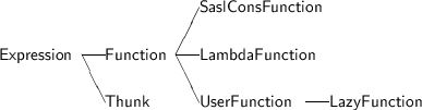
The SASL interpreter is largely constructed by removing features from the Scheme interpreter, such as while loops and so on, and changing the implementation of the cons function to add delayed evaluation. Figure 5.1 shows the class hierarchy for the classes added in this chapter.
Delayed evaluation is provided by adding a new expression type, called the thunk. Figure 5.1 shows the data structure used to represent this type of value. Every thunk maintains a boolean value indicating whether the thunk has been evaluated yet, an expression (representing either the unevaluated or evaluated expression, depending upon the state of the boolean �ag), and a context in which the expression is to be evaluated. Thunks print either as three dots, if they have not yet been evaluated, or as the printed representation of their value, if they have.
Here we �nally see an overridden de�nition for the method touch. You will recall that this method was de�ned in Chapter 1, and that all other expressions merely return their value as the result of this expression. Thunks, on the other hand, will evaluate themselves if touched, and then return their new evaluated result. With the addition of this feature many of the de�nitions we have presented in earlier chapters, such as the de�nitions of car and cdr, hold equally well when given thunks as arguments.
Since thunks can represent lists, symbols, integers and so on, the predicate methods isSymbol and the like must be rede�ned as well. If the thunk represents an evaluated value, these simply return the result of testing that value (Figure 5.3).
The SASL cons function di�ers from the Scheme version in producing a list node containing a pair of thunks, rather than a pair of values (Figure 5.5). Class SaslConsFunction must now be a subclass of Function and not BinaryFunction, because it must grab its arguments before they are evaluated. Thus it must itself check to see that only two arguments are passed to the function.
User de�ned functions must be provided with lazy evaluation semantics as well. This is accomplished by de�ning a new class LazyFunction (Figure 5.6). Lazy functions act just like user functions from previous chapters, only they do not evaluate their arguments. Thus the function body is evaluated by the method apply, rather than passing the evaluated arguments on to the method applyWithArgs. The lambda function from the previous chapter is modi�ed to produce an instance of LazyFunction, rather than UserFunction.
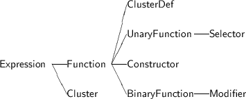
The CLU interpreter is created by introducing a new datatype, the cluster, and three new types of functions. Constructors create new instances of a cluster, selectors access a portion of a cluster state, and modi�ers change a portion of a cluster state. Figure 6.1 shows the class hierarchy for the classes added in this chapter.
A cluster simply encapsulates a series of names and values, hiding them from normal examination. The most natural way to do this is for a cluster to maintain an environment (Figure 6.1). The predicate isCluster returns this environment value.
To create a cluster requires a constructor function. The constructor is provided with a list of names of the elements in the internal representation of the cluster, and simply insures that the arguments it is provided with match in number of the names it maintains.
To access or modify the elements of a constructor requires functions called selectors or modi�ers. Each of these maintain as their state the name of the �eld they are responsible for. When invoked with a constructor, the access or change their given �eld.
It thus remains only to give the (rather lengthy) de�nition of the function that generates constructor information from the textual description. (We do not say generates clusters themselves, for that is the responsibility of the constructor functions). This function is shown in Figure 6.3. It rips apart a cluster de�nition and does the right things (need a better description here, but I don't have time to write it now). (Need to point out that cluster functions have an internal and an external name, and these are put of di�erent environments). (I suppose an alternative would have been to introduce a new datatype for two part names, which when evaluated would look up their second part in the cluster provided by their �rst part).
As with chapter 3, with the Smalltalk interpreter I have also made a number of changes. These include the following:
((x < y) if (set z x) (set z y))
A class hierarchy for the classes added in this chapter is shown in Figure 7.1.
An object is an encapsulation of behavior and state. That is, an object maintains, like a cluster, certain state information accessible only within the object. Similarly objects maintain a collection of functions, called methods, that can be invoked only via message passing. Internally, both these are represented by environments (Figure 7.1). The methods environment contains a collection of functions, and the data environment contains a collection of internal variables. Objects are declared as a subclass of function so that normal function syntax can be used for message passing. That is, a message is written as
(object message arguments)
Methods are similar to conventional functions (and are thus subclasses of UserFunction) in that they have an argument list and body. Unlike conventional functions they have a receiver (which must always be an object) and the environment in which the method was created, as well as the environment in which the method is invoked. Thus methods de�ne a new message doMethod that takes these additional arguments.
A subtle point to note is that the creation environment in normal functions is captured when the function is de�ned. For objects this environment cannot be de�ned when the methods are created, but must wait until a new instance is created. Our implementation waits even longer, and passes it as part of the message passing protocol.
The mechanism of message passing is de�ned by the function apply in class Object (Figure 7.2). Messages require a symbol for the �rst argument, which must match a method for the object. This method is then invoked. Similarly Figure 7.2 shows the execution of normal methods (that is, those methods other than the ones provided by the system). The execution context is set for the method, and the receiver is added as an implicit �rst argument, called self in every method. The method is then invoked as if it were a conventional function.
Classes are simply objects. As such, they respond to certain messages. In our Smalltalk interpreter there are initially two classes, Object and Integer. The class Object is a superclass of Integer, and is typically the superclass of most user de�ned classes as well. There are initially three messages that classes respond to:
(set Foo (Object subclass x y z))
which creates a new class with three instance variables, and assigns this class to the variable Foo. Subclasses can also access instance variables de�ned in classes.
It is legal to subclass from class Integer, although the results are not useful for any purpose.
(set newfoo (Foo new))
Although the class Integer responds to the message new, no useful value is returned. (Real Smalltalk has something called metaclasses that can be used to prevent certain classes from responding to all messages. Our Smalltalk doesn't).
(Integer method square () (self * self))
Classes are represented in the same format as other objects. They act as if they held two instance variables; names, which contains a list of instance variable names for the class, and methods, which contains the table of method de�nitions for the class. Note that these are held in the data area for the class. (A picture might help here...).
The implementation of the method subclass is shown in Figure 7.3. The instance variables for the parent class is obtained, and the new instance variables for the class added to them. Inheritance is implemented by creating a new empty method table, but having it point to the method table for the parent class. Thus a search of the method table for the newly created class will automatically search the parent class if no overriding method is found. These two values are inserted as data values in the new class object. The methods a class responds to will be exactly the same as those of the parent class (thus all classes respond to the same messages).
The implementation of the method new, shown in Figure 7.5, gets the list of instance variables associated with the class. A new environment is then created that assigns an empty value to each variable. Using the method table stored in the data area for the class object a new object is then created.
The method used to respond to the method command is shown in Figure 7.6. This is very similar to the function used to break apart the de�ne command in Chapter 1. The only signi�cant di�erence includes the addition of the receiver self as an implicit �rst parameter in the argument list, and the fact that the function is placed in a method table, rather than in the global environment.
Symbols in Smalltalk have no property other than they evaluate to themselves, and are guaranteed unique. They are easily implemented by subclassing the existing class Symbol (Figure 7.7), and modifying the reader/parser to recognize the tokens. (Unlike symbols in real Smalltalk, our symbols are not objects and will not respond to any messages).
Integers are also rede�ned as objects, and a built-in method IntegerBinaryMethod (Figure 7.8), similarly to IntegerBinaryFunction, is created to simplify the arithmetic methods.
Control �ow is implemented as a message to integers. (In real Smalltalk control �ow is implemented as messages, but to di�erent objects). If the receiver is zero the �rst argument to the if method is returned, otherwise the second argument is returned.
The Smalltalk reader subclasses the reader class so as to recognize integers and symbols (Figure 7.10).
To initialize the interpreter we must create the objects Object and Integer. (Need more explanation here, but I'll just give the code for now).
As with chapters 3 and 7, I have in this chapter taken great liberties with the syntax used by Kamin in his interpreter. However, unlike chapters 3 and 7, where my intent was to make the interpreters closer in spirit to the original language, my intent here is to simplify the interpreter. Speci�cally, I wanted to build on the base interpreter, just as we have done for all other languages. I am able to do this by adopting continuations as the fundamental basis for my implementation, and by basing the code on slightly di�erent primitives.
The language used by this interpreter has the following characteristics:
For example, suppose sam is the father of alice, and alice is the mother of sally. We might encode this in a parent database as follows:
The query statement can then be used to ask queries of the database. For example, we can �nd out who is the parent of alice as follows:
Or we can �nd the child of alice with the following:
If we ask a question that does not have an answer, the response not-ok is printed.
Prolog style rules can be introduced using the same form we have been using for functions.
There is no built-in way to force a relation to cycle through all alternatives. However, this is easily accomplished by making a relation that will always fail, for example trying to unify apples with oranges:
We can then use this to print out all the parents in our database. Notice that not-ok is printed, since we eventually fail.
Note - although it might appear the use of and's and or's is more powerful than writing rules in horn clauses, in fact they are identical; although horn clauses will often require the introduction of unnecessary names. I myself �nd this formulation more natural, although I'm not exactly unbiased.
Uni�cation of two unknown symbols works as expected. If any symbol subsequently becomes de�ned, the other is de�ned as well.
I will divide the discussion of the implementation into three parts. These are uni�cation, symbol management, and backtracking.
Uni�cation is the basis for logic programming. Using uni�cation, unbound variables can be bound together. As we saw in the last example, this is more than simple assignment. If two unknown variables are uni�ed together and subsequently one is bound, the other should be bound also. Uni�cation also di�ers from assignment in that it can be \undone" during the process of backtracking.
Uni�cation is most easily implemented by introducing a level of indirection. Prolog values will be represented by a new type of expression, called PrologValue (Figure 8.1). Instances of this class maintain a data value, which is either unde�ned (that is, null), a symbol, or another prolog value. The prolog reader is modi�ed so as to return a prolog value were formerly a symbol was returned. (Also the reader will no longer recognize integers, which are not used in our simpli�ed interpreter).
A prolog value that contains a symbol is used to represent the prolog symbol of the same name. A prolog value that contains an empty data value represents a currently unbound value. Finally a prolog value that points to another prolog value represents the uni�cation of the �rst value with the second. Whenever we need the value of a prolog symbol, we �rst run down the chain of indirections to get to the bottom of the sequence. (This is done automatically by the overridden method isSymbol, which will yield the symbol value behind arbitrary levels of indirection if a prolog value represents a symbol.)
The uni�cation algorithm is shown in Figure 8.2. For reasons we will return to when we discuss backtracking, the algorithm takes three arguments. The �rst is a reference to a pointer to a prolog value. If the uni�cation process changes the value of either the the two other arguments, the pointer in the �rst argument is set to the altered value.
The uni�cation process divides naturally into three parts. If either argument is unde�ned, it is changed so as to point to the other arguments. This is true regardless of the state of the other argument. This is how two unde�ned variables can be uni�ed - the �rst is set to point to the second. If the second is subsequently changed, the �rst will still indirectly point to the new value. Suppose it is, however, the �rst that is subsequently changed? In that case the next portion of the uni�cation algorithm is entered. If both arguments are de�ned and either one is an indirection, then we simply try to unify the next level down in the pointer chains. (Note: Lots of pictures would make this clearer, but I don't have time right now..). If neither argument is unde�ned nor an indirection, they both must be symbols. In that case, uni�cation is successful if and only if they have the same textual representation.
The only signi�cant problem here is that symbolic constants must evaluate to themselves and that symbolic variables can be introduced without declaration. We see the latter in sequences such as:
Here the variable Z suddenly appears without prior use. The solution to both of these problems is found in the code used to respond to the eval request for a Prolog value. This code is shown in Figure 8.3. The virtual method isSymbol runs down any indirection links, returning the symbol data value if the last value in a chain of indirections represents a symbolic constant. If a symbol is found, we �rst look to see if the symbol is bound in the current environment. If so we simply return its binding1 . If not, if the symbol begins with a lower case letter it evaluates to itself, and so we simply return it. If it is not a symbolic constant, than it is a new symbolic variable, and we add a binding to the current environment to indicate that the value is so-far unde�ned. Thus new symbols are added to the current environment as they are encountered, instead of generating error messages as they did in previous interpreters.
The seem to be two general approaches to implementing logic programming languages. The technique used by most modern prolog systems is called the WAM, or Warren Abstract Machine. The WAM performs backtracking by not popping the activation frame stack when a procedure is terminated, and saving enough information to restart the procedure in a record called the \choice point". Since in our interpreters calling a function is performed by recursively calling evaluation routines inside the interpreter, the activation stack for the users program is held in part in the activation stack for the interpreter itself. Thus it is di�cult for us to manipulate the activation record stack directly. The alternative technique, which is actually historically older, is to build up an unevaluated expression that represents what it is you want to do next before you ever start execution. This is called a continuation, and we were introduced to this idea in the chapter on Scheme. When we are faced with a choice, we can then try one alternative and the continuation, and if that doesn't work try the next.
In general continuations are simply arbitrary expressions representing \what to do next". In our case they will always return a boolean value, indicating whether they are to be considered successful or not. We will sometimes refer to the continuation as the \future", since it represents the calculation we want to perform in the future.
In order to illustrate how backtracking can be implemented using continuation, let us consider the following invocation of our family database:
There are two important points to note. The �rst is that the general approach will be a two step process, construct the future that represents the calculation we want to do, then do it. The second point is that the details are exceedingly messy; you should be eternally grateful that it is the computer that is performing this task, and not you.
To begin, the continuation that represents what it is we want to do after evaluating the query is the null continuation, an expression that merely returns true. In order to try to keep track of the multiple levels of evaluation, let us write this as follows:
This says that we want to evaluate the and relation, and then do the calculation given by the bracketed expression.
Consider now the meaning of and. The and expression should evaluate the �rst relation, and if successful evaluate the second, and �nally if that is successful evaluate the future given to the original expression. What then is the \future" of the �rst relation? It is simply the second relation and the original future. That is, the calculation we want to perform if the �rst relation is successful is simply the following:
We can wrap this in a bracket in order to make a continuation in our form out of it. Using this as the future for the �rst relation gives us the following:
We are in e�ect turning the calculation inside out. We have replaced the and conjunction with a list of expressions to evaluate in the future.
The invocation of the grandparent relation causes the expression to be replaced by the function de�nition, with the arguments suitably bound to the parameters. That is, the e�ect is the same as:2
We have already analyzed the meaning of the and relation. The future we want to provide for the �rst relation is the expression yielded by:
As before, we can expand the invocation of the parent relation by replacing it by its de�nition, making suitable transformations of the argument values.
The or relation should try each alternative in turn, passing it as the future the continuation passed to the or. If any is successful we should return success, otherwise the or should fail. Thus we can distribute the future to each clause of the or, and rewrite it as follows:3
If we perform the already-de�ned transformations on the and relations we obtain the following:
Recall that this was all performed just to construct the continuation for the �rst clause in an earlier expression. Thus the expression we are now working on is as follows:
We before, we can expand the call on parent by its de�nition:4
Once again distributing the future along each argument of the or expression yields:
Performing yet one more time the transformations on the and relations yields:
This is the �nal continuation that is constructed by the query expression. The most important feature of this expression is that it can be evaluated in a forward fashion, without backtracking. Having generated it, the next step is execution. Contrast this with the description we provided earlier. First an attempt is made to unify the symbols sam and alice. This fails, and thus the continuation for the �rst conditional is ignored. Next an attempt is made to unify the symbols sam and sam. This is successful, and thus we evaluate the continuation to the next expression. The continuation uni�es Z and alice, binding the left-hand variable to the right-hand symbol. The continuation for that expression then trys to unify Z and alice, which is successful. Thus variable A is bound to sally, and is printed.5
Having described the general approach our interpreter will follow, we will now go on to provide the speci�c details.
Our continuations are built around a new datatype, which we will call the Continuation. A continuation should be thought of as an unevaluated boolean expression. The continuation performs some action, which may or may not succeed. The success of the action is indicated by the boolean value returned. The class Continuation is shown in Figure 8.4. The routine used to invoke a relation is the virtual method withContinuation, which takes as argument the future for the continuation.
Initially there is nothing we want to do in the future. So the initial relation simply ignores its future, does nothing and always succeeds. In fact, in our implementation we maintain a global variable called nothing to hold this relation. You can think of this variable as maintaining the relation [ true ].
The simplest relation is the one correspond to the command to print. When a print relation is created, the value it will eventually print is saved as part of the relation. If the argument passed to the print relation is, following any indirection, a symbolic value than it is printed out, and the future passed to the relation is invoked. If the argument was not a symbol, or if the future calculation was unsuccessful, then the relation indicates its failure by returning a zero value. The code to accomplish this is shown in Figure 8.5.
Next let us consider the uni�cation relation. As with printing, the two expressions representing the elements to be uni�ed are saved when the uni�cation operator is encountered during the construction of the future. When we invoke this relation the two arguments are uni�ed, using the algorithm we have previously described. If this uni�cation is successful the relation attempts to evaluate the future continuation. Only if both of these are successful does the relation return one. If either the uni�cation fails or the future fails then the binding created by the unify procedure is undone and failure is reported. (Figure 8.6).
Next consider the or relation (Figure 8.7). This relation takes some number of argument relations. It tries each in turn, followed by the future it has been provided with. If any succeeds then it returns a true value, otherwise if all fail it returns a failure indication.
It is in the or relation that backtracking occurs, although it is di�cult to tell from the code shown here. Recall that the uni�cation algorithm undoes the e�ect of any assignment if the continuation passed to it cannot be performed. Thus the future that is passed to the or relation may be invoked several times before we �nally �nd a sequence of assignments that works.
The and relation is perhaps the most interesting. To understand this let us �rst take the case of only two relations, which we will call rel1 and rel2. Let f represent the continuation we wish to evaluate if the and relation is successful. What then is the future we should pass to the �rst relation? If the �rst relation is successful, we want to evaluate the second relation and then the continuation. Thus the future for the �rst relation is the composition of the future for the second relation and the original continuation. This can be written as rel2(f), but we must make it into a continuation, we we create a new datatype called a CompositionContinuation. Interestingly, this composition relation ignores its continuation, and is merely executed for its side e�ect. This is the future we want to pass to the �rst relation. We can generalize this to any number of arguments. For example the and of three arguments should return the value produced by rel1([rel2([rel3([f])])]), and so on.
The composition step is performed by the datatype ComposeContinuation, shown in Figure 8.8. As in our description, when a composition relation is evaluated it ignores the future it is provided with and merely returns the �rst relation provided with the second relation as its future. Having de�ned this, the and relation (Figure 8.9) is a simple recursive invocation.
You may have noticed that the class Continuation is not a subclass of class Function, and yet we have been discussing continuations as if they were functions. This is easily explained. Recall that evaluating a relation in our approach is a two-step process. First the relation is constructed, and in the second step the future is brought to life. The functional parts of each of the four relation-building operations are concerned only with the �rst part of this task. These are all trivial functions, shown in Figure 8.10.
The query statement is responsible for the construction and execution of the continuation corresponding to its argument. The function implementing the query statement is shown in Figure 8.11. A new environment is created prior to evaluating the arguments so that bindings created for new variables do not get entered into the global environment. Then the continuation is constructed, simply by evaluating the argument. If this process is successful, the continuation is then executed, and if the continuation is successful the symbol ok is yielded as the result (and thus printed by the read-eval-print loop). If the continuation is not successful the symbol not-ok is generated.
The initialization function for the prolog interpreter (Figure 8.12) is one of the shortest we have seen. It is only necessary to create the two commands de�ne and query, and the four relational-building operations.
The following list represents a few of the ideas that occurred to me as I was developing these interpreters for how things might be done di�erently. These are presented in no particular order. (Nor as any particularly grave criticism of the Kamin interpreters - I still think the book as a whole is very good).